An Overview of Undergraduate Bayesian Education

Talk at Statistical Sciences Applied Research and Education Seminar
University of Toronto and CANSSI Ontario

Mine Dogucu
University of California Irvine

2023-12-11

Outline

• Why?
• Research Study
• Recommendations
• Example
• Resources

Why?

p-values

Q: Why do so many colleges and grad schools teach p = 0.05?

A: Because that’s still what the scientific community and journal editors use.

Q: Why do so many people still use p = 0.05?

A: Because that’s what they were taught in college or grad school.

George Cobb as quoted in The ASA’s Statement on p-Values: Context, Process, and Purpose

“In 1985 only about 10% of JASA Applications and Case Studies articles used Bayesian methods.

In 2022 plus half of 2023, that percentage has changed. It is now 49%.”

Jeff Witmer, To Bayes or Not to Bayes – Is There Any Question? Talk at Joint Statistical Meetings, 2023

• intuitive

• draws a more complete picture of statistics from both philosophical and application perspectives

• prepares students for their future career

• statistics and computing can be taught in a harmonious way

Examples

Witmer, J. (2017), Bayes and MCMC for Undergraduates, The American Statistician, 71, 259–264. DOI: 10.1080/00031305.2017.1305289.

Hu, J. (2020), A Bayesian Statistics Course for Undergraduates: Bayesian Thinking, Computing, and Research, Journal of Statistics Education, 28, 229–235.

Hoegh, A. (2020), Why Bayesian Ideas Should be Introduced in the Statistics Curricula and How to do so Journal of Statistics Education, 28, 222–228. DOI: 10.1080/10691898.2020.1841591.

Hu, J., and Dogucu, M. (2022), Content and Computing Outline of Two Undergraduate Bayesian Courses: Tools, Examples, and Recommendations, Stat, 11, e452. DOI: 10.1002/sta4.452.

Research

Dogucu, M. & Hu, J. (2022) The Current State of Undergraduate Bayesian Education and Recommendations for the Future. The American Statistician, 74(2), 405-413.

The authors gratefully acknowledge data collection support of Feiyi Sun.

We wanted to know how commonly Bayesian statistics is taught at the undergraduate level as a course and how it is taught.

Methods

• We collected data on all universities with a ranking of 100 or higher (i.e., better ranking) and liberal arts colleges with a ranking of 50 or higher based on U.S. News rankings

• We searched the word “Bayesian” in course catalogs of the selected institutions spanning two academic years, from Fall 2019 to Summer 2021.

• We only tracked courses that contain the word “Bayesian” in the title of the course.

Data

• the department the Bayesian course is offered

• whether the course is cross-listed for undergraduate and graduate enrollment

• whether it is part of any major as an elective or a required course.

• prerequisites

• course content (as seen in syllabi)

Results

Among the 152 high-ranking institutions, we identified 46 institutions that offer a Bayesian course.

In total, we have identified 51 Bayesian courses and note that 5 universities have two Bayesian courses.

Breaking down by institution type, it is 12% of the colleges (6 out of 50) and 39% of the universities (40 out of 102), respectively.

Of the 45 courses offered at universities, 60% are cross-listed between undergraduate and graduate programs.

Departments

• 51% are offered in statistics departments
• 7.8% in computer science departments
• 2% in math departments

There are also many departments which are at the intersection of statistics, mathematics, computer science, and/or data science. These departments offer 17.6% of the identified Bayesian courses.

The remaining 21.6% courses are taught in various departments such as physics, psychology, ecology, evolution and marine biology and two of which were cross-listed between multiple departments.

Majors

Prerequisites

Prerequisites - Math

• 43% of the 51 Bayesian courses have three calculus courses as prerequisites

• 29% require two calculus courses

• 10% require one calculus course

• 16% do not require calculus courses at all.

37% courses require linear algebra

Prerequisites - Computing

While 33% of the 51 Bayesian courses mention some sort of computing prerequisite, not all of these mentions are prerequisite courses.

Courses: introductory computer programming courses, statistical computing, R for data science, data science with R, R programming, data structures, computational thinking and doing, SAS programming.

Some mention a computing software. e.g., “R recommended,” “familiarity with R,” “basics of R programming required,” “some acquaintance with fundamentals of computer programming,” “familiarity with some programming language or numerical computing environment.”

Prerequisites - Probability and Statistics

Content

Textbooks

Recommendations

Expand the Access to Bayesian Courses

• Offer an undergraduate course in Bayesian statistics.

• Reduce the number of prerequisites.

• Include Bayesian modules as part of existing courses.

Make Bayesian Courses a Part of the Majors

• Consider making the Bayesian course required for statistics and data science majors.

• If the Bayesian course is an elective, then make it a highly recommended elective.

• Consider making the Bayesian course an elective for majors beyond the statistical, mathematical, and computational sciences.

Balance Statistics with Computing

• Introduce simulation-based learning early in the course.

• Encourage students to write self-coded MCMC algorithms for relatively simple multi-parameter models.

• If the course puts equal emphasis on computing and modeling, consider adopting one of the popular probabilistic programming languages for Bayesian model estimation through MCMC.

• If the course has a slightly stronger emphasis on modeling over computing, consider introducing one of the wrapper packages for Stan for its simpler posterior summary procedure.

Example

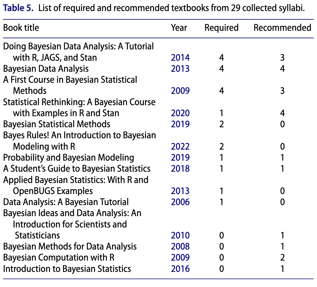
Johnson, A. A., Otts, M. & Dogucu, M. (2022) Bayes Rules! An Introduction to Applied Bayesian Modeling

{bayesrules}

• Bayesian Foundations
• Posterior Simulation & Analysis
• Regression and Classification
• Hierarchical Models

Bayes’ Rule

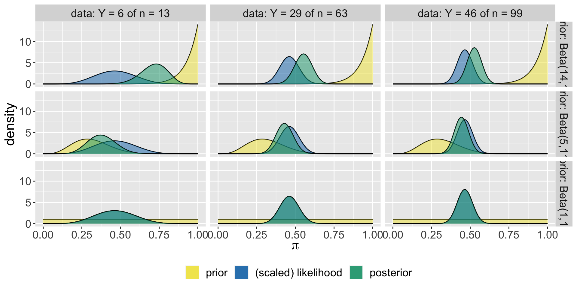
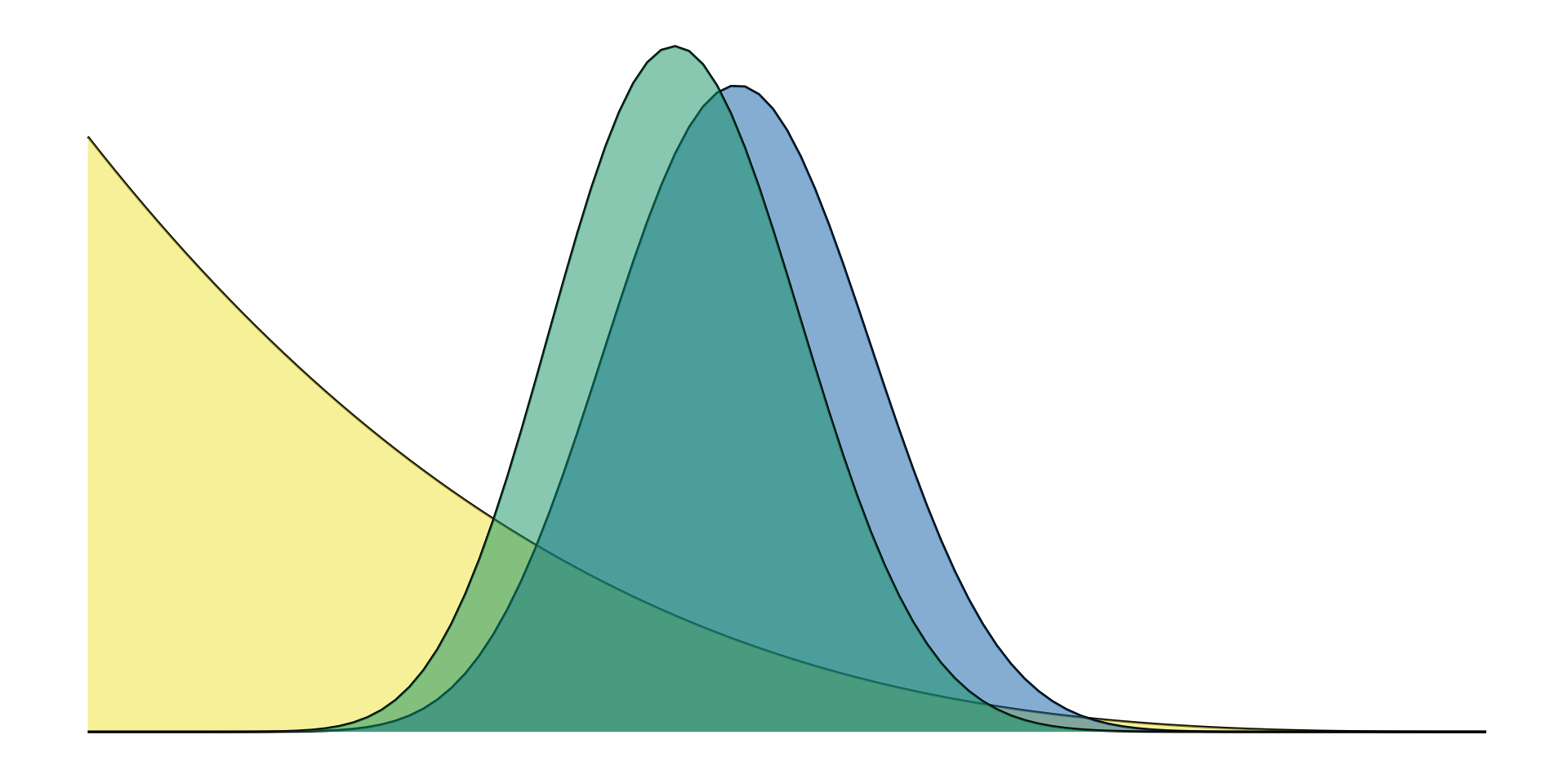
The Beta-Binomial Bayesian Model

Balance and Sequentiality in Bayesian Analysis

Conjugate Families

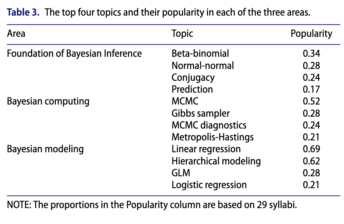
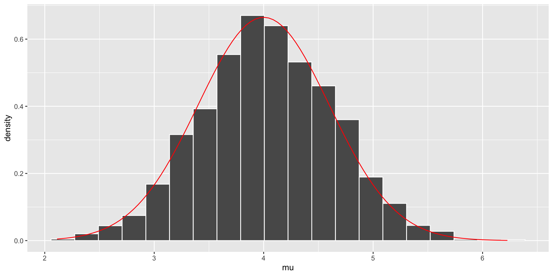
Grid Approximation

The Metropolis-Hastings Algorithm

Posterior Estimation

Posterior Hypothesis Testing

Posterior Prediction

Normal Regression

Poisson and Negative Binomial Regression

Logistic Regression

Naive Bayes Classification

Normal hierarchical models without predictors

Normal hierarchical models with predictors

Non-Normal Hierarchical Regression & Classification

Dogucu, M. & Johnson A. (2022) Supporting Bayesian Modeling with Visualizations. In S. Peters (Ed) Proceedings of the 11th International Conference on Teaching Statistics. Rosario, Argentina.

one_mh_iteration <- function(w, current){
 # STEP 1: Propose the next chain location
 proposal <- runif(1, min = current - w, max = current + w)
  
 # STEP 2: Decide whether or not to go there
 proposal_plaus <- dnorm(proposal, 0, 1) * dnorm(6.25, proposal, 0.75)
 current_plaus  <- dnorm(current, 0, 1) * dnorm(6.25, current, 0.75)
 alpha <- min(1, proposal_plaus / current_plaus)
 next_stop <- sample(c(proposal, current), 
  size = 1, prob = c(alpha, 1-alpha))
  
 # Return the results
 return(data.frame(proposal, alpha, next_stop))
}

mh_tour <- function(N, w){
  # 1. Start the chain at location 3
  current <- 3
  # 2. Initialize the simulation
  mu <- rep(0, N)
  # 3. Simulate N Markov chain stops
  for(i in 1:N){    
    # Simulate one iteration
    sim <- one_mh_iteration(w = w, current = current)
    
    # Record next location
    mu[i] <- sim$next_stop
    
    # Reset the current location
    current <- sim$next_stop
  }
  
  # 4. Return the chain locations
  return(data.frame(iteration = c(1:N), mu))
}

set.seed(84735)
mh_simulation_1 <- mh_tour(N = 5000, w = 1)

Resources

Undergraduate Bayesian Education Resources

Undergraduate Bayesian Education Network

STATS 115 at University of California Irvine

Bayes BATS for Advancing Bayesian Thinking in STEM

Acknowledgments

Supported by NSF HDR DSC award #2123366

Supported by NSF IUSE: EHR program with award #2215879

QUESTIONS?

minedogucu.com
mdogucu
MineDogucu
mastodon.social/@MineDogucu
minedogucu