Rows: 100
Columns: 10
$ artist            <fct> Ad Gerritsen, Kirstine Roepstorff, Lisa Baumgardner,…
$ country           <fct> dutch, danish, american, american, american, canadia…
$ birth             <fct> 1940, 1972, 1958, 1952, 1946, 1927, 1901, 1941, 1920…
$ death             <fct> 2015, NA, 2015, NA, NA, 1966, 1971, NA, 2007, NA, NA…
$ alive             <lgl> FALSE, TRUE, FALSE, TRUE, TRUE, FALSE, FALSE, TRUE, …
$ genx              <lgl> FALSE, TRUE, FALSE, FALSE, FALSE, FALSE, FALSE, FALS…
$ gender            <fct> male, female, female, male, male, male, male, male, …
$ count             <int> 1, 3, 2, 1, 1, 8, 2, 1, 1, 5, 1, 2, 1, 1, 21, 16, 1,…
$ year_acquired_min <fct> 1981, 2005, 2016, 2001, 2012, 2008, 2018, 1981, 1949…
$ year_acquired_max <fct> 1981, 2005, 2016, 2001, 2012, 2008, 2018, 1981, 1949…Posterior Inference and Prediction
Dr. Mine Dogucu
The notes for this lecture are derived from Chapter 8 of the Bayes Rules! book
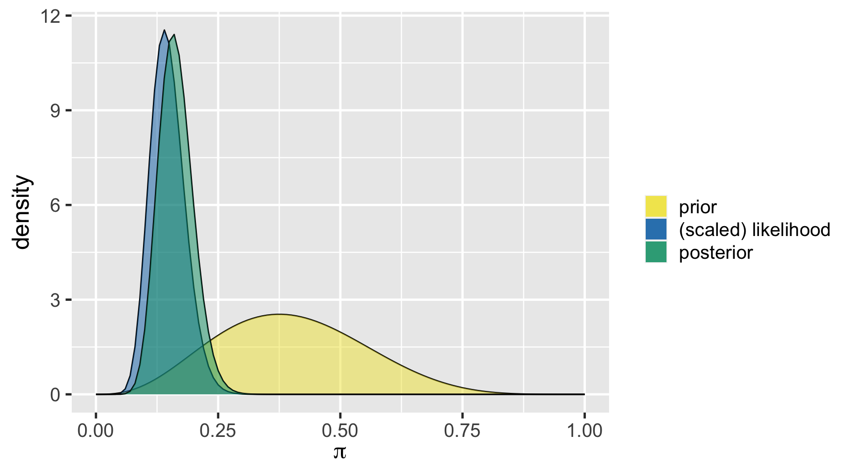
\[Y|\pi \sim \text{Bin}(100, \pi)\]
\[\pi \sim \text{Beta}(4, 6)\]
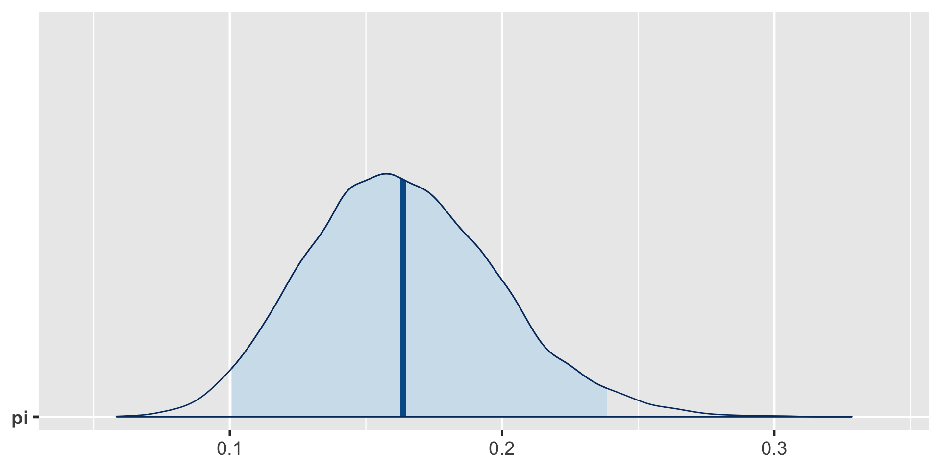
\[\begin{split} Y | \pi & \sim \text{Bin}(100, \pi) \\ \pi & \sim \text{Beta}(4, 6) \\ \end{split} \;\;\;\; \Rightarrow \;\;\;\; \pi | (Y = 14) \sim \text{Beta}(18, 92)\]
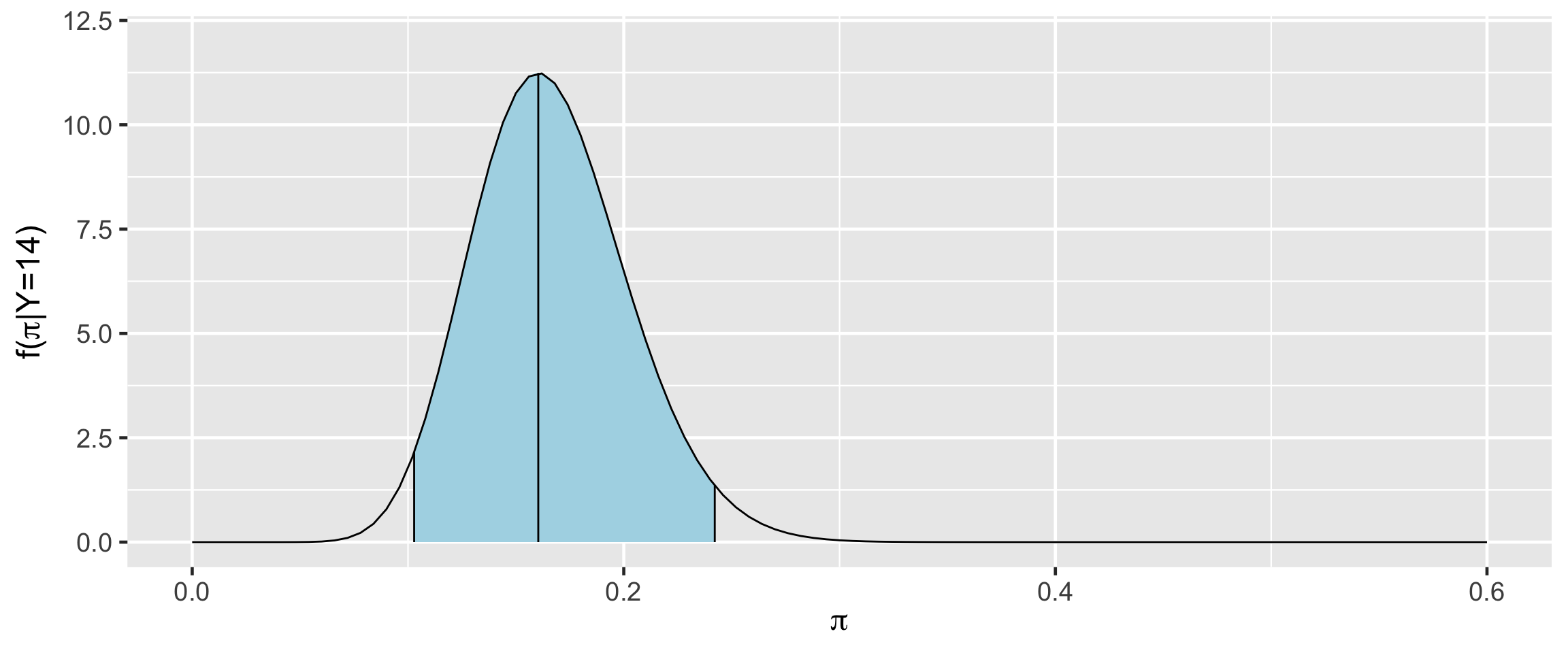
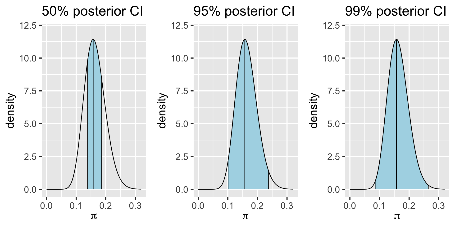
95% Posterior Credible Interval (CI)
0.025th & 0.975th quantiles of the Beta(18,92) posterior
\(\int_{0.1}^{0.24} f(\pi|(y=14)) d\pi \; \approx \; 0.95\)
\[\begin{split} H_0: & \; \; \pi \ge 0.20 \\ H_a: & \; \; \pi < 0.20 \\ \end{split}\]
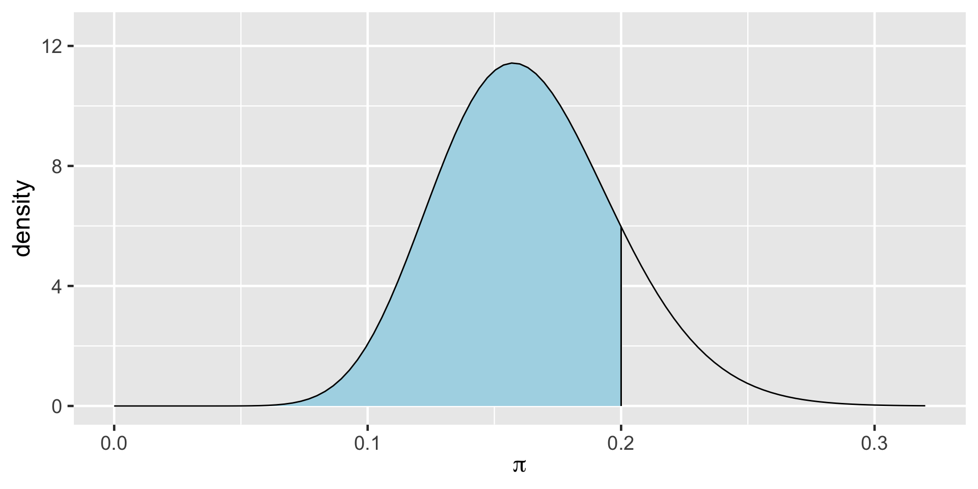
\[\text{Posterior odds } = \frac{P(H_a \; | \; (Y=14))}{P(H_0 \; | \; (Y=14))} \approx 5.62 \]
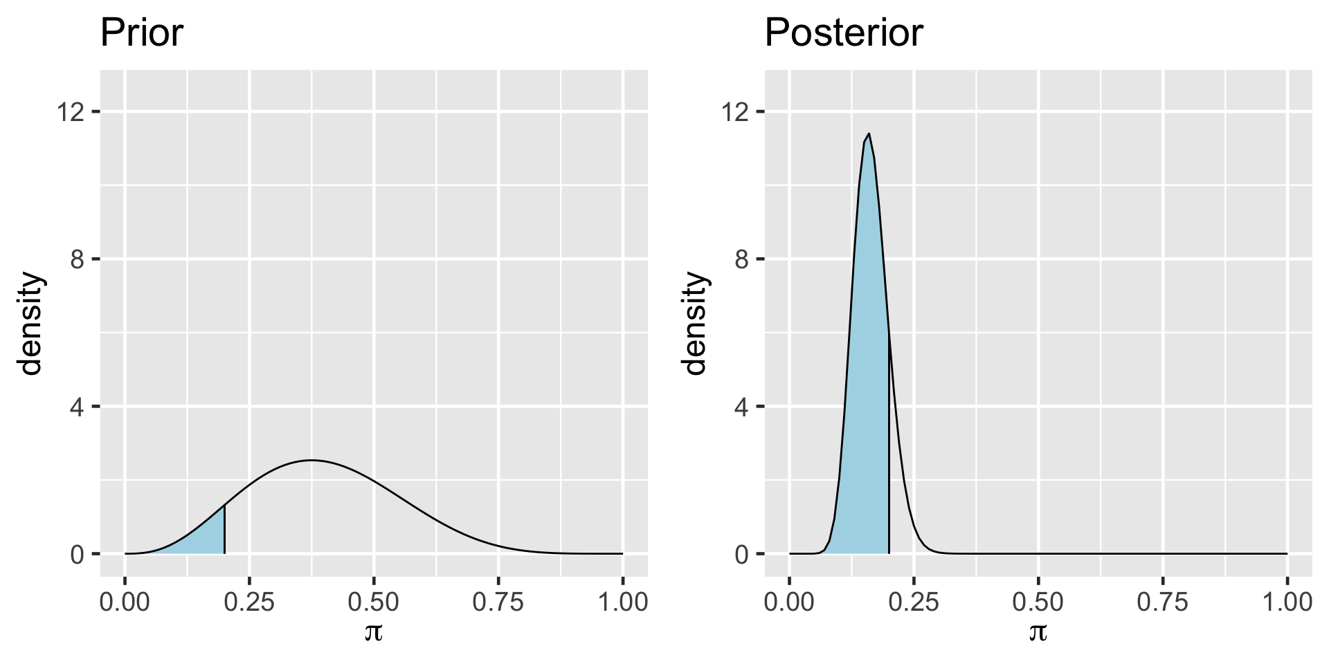
\[P(\pi<0.20)\]
The Bayes Factor (BF) compares the posterior odds to the prior odds, hence provides insight into just how much our understanding about Gen X representation evolved upon observing our sample data:
\[\text{Bayes Factor} = \frac{\text{Posterior odds }}{\text{Prior odds }}\]
Bayes Factor
In a hypothesis test of two competing hypotheses, \(H_a\) vs \(H_0\), the Bayes Factor is an odds ratio for \(H_a\):
\[\text{Bayes Factor} = \frac{\text{Posterior odds}}{\text{Prior odds}} = \frac{P(H_a | Y) / P(H_0 | Y)}{P(H_a) / P(H_0)} \; .\]
As a ratio, it’s meaningful to compare the Bayes Factor (BF) to 1. To this end, consider three possible scenarios:
- BF = 1: The plausibility of \(H_a\) didn’t change in light of the observed data.
- BF > 1: The plausibility of \(H_a\) increased in light of the observed data. Thus the greater the Bayes Factor, the more convincing the evidence for \(H_a\).
- BF < 1: The plausibility of \(H_a\) decreased in light of the observed data.
Two-sided Tests
\[\begin{split} H_0: & \; \; \pi = 0.3 \\ H_a: & \; \; \pi \ne 0.3 \\ \end{split}\]
\[\text{Posterior odds } = \frac{P(H_a \; | \; (Y=14))}{P(H_0 \; | \; (Y=14))} = \frac{1}{0} = \text{ nooooo!}\]
library(rstan)
# STEP 1: DEFINE the model
art_model <- "
data {
int<lower=0, upper=100> Y;
}
parameters {
real<lower=0, upper=1> pi;
}
model {
Y ~ binomial(100, pi);
pi ~ beta(4, 6);
}
"
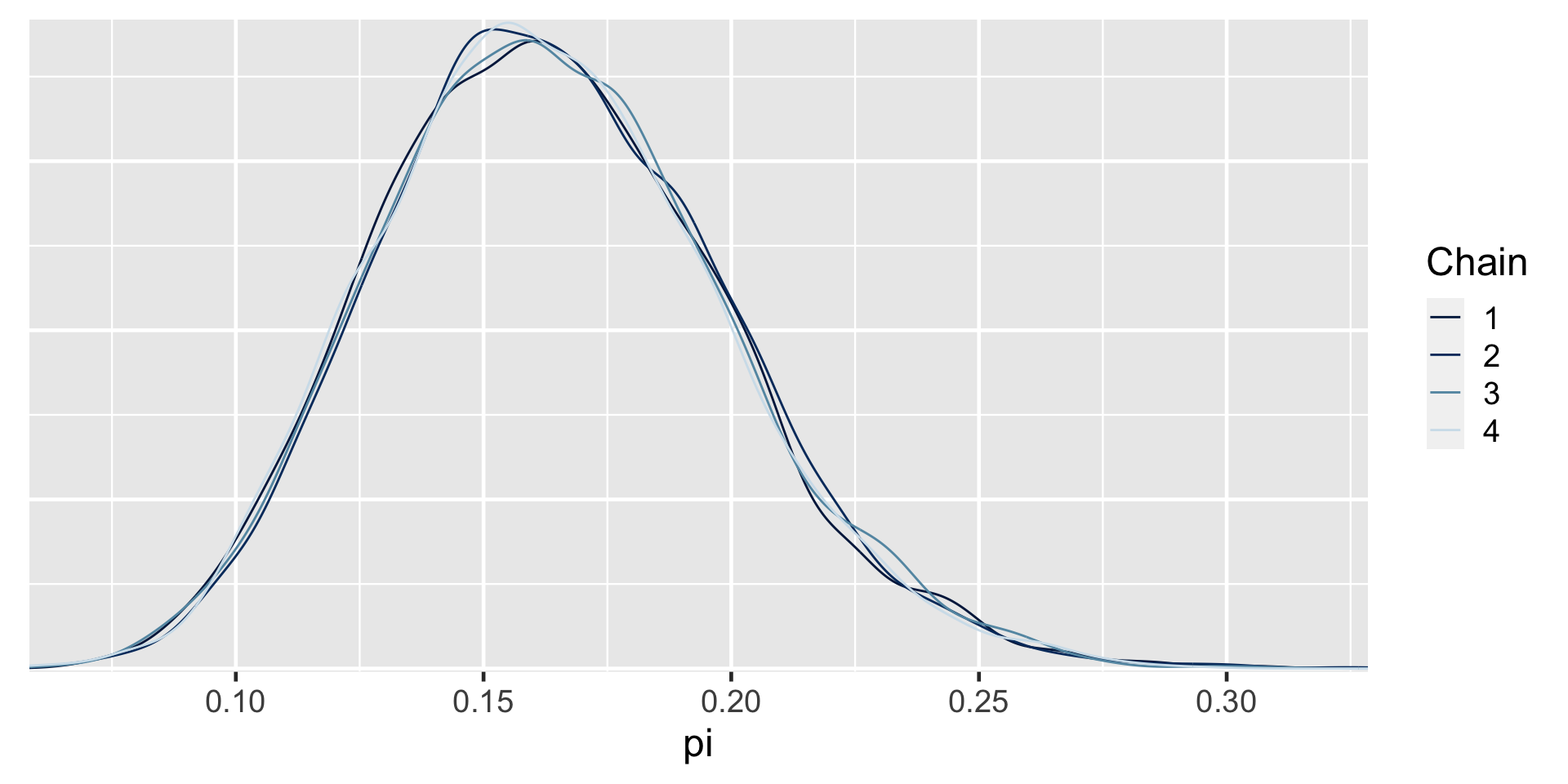
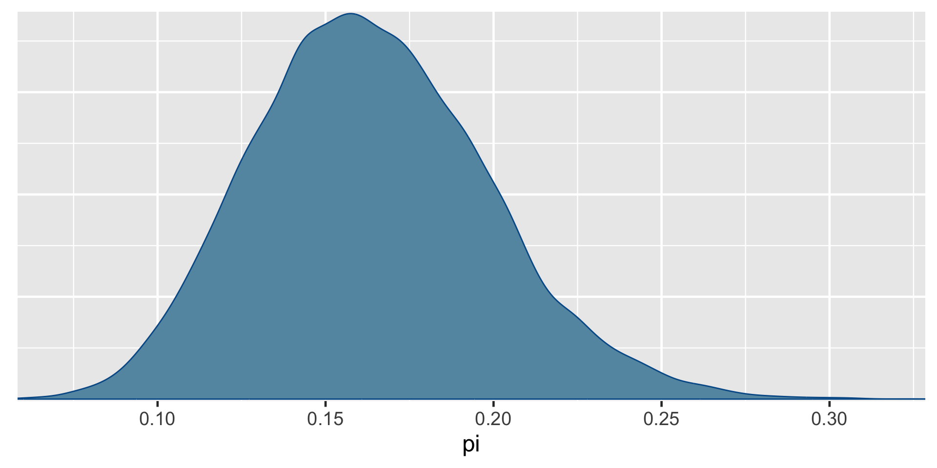
# STEP 2: SIMULATE the posterior
art_sim <- stan(model_code = art_model, data = list(Y = 14),
chains = 4, iter = 5000*2, seed = 84735)
SAMPLING FOR MODEL 'anon_model' NOW (CHAIN 1).
Chain 1:
Chain 1: Gradient evaluation took 1.1e-05 seconds
Chain 1: 1000 transitions using 10 leapfrog steps per transition would take 0.11 seconds.
Chain 1: Adjust your expectations accordingly!
Chain 1:
Chain 1:
Chain 1: Iteration:    1 / 10000 [  0%]  (Warmup)
Chain 1: Iteration: 1000 / 10000 [ 10%]  (Warmup)
Chain 1: Iteration: 2000 / 10000 [ 20%]  (Warmup)
Chain 1: Iteration: 3000 / 10000 [ 30%]  (Warmup)
Chain 1: Iteration: 4000 / 10000 [ 40%]  (Warmup)
Chain 1: Iteration: 5000 / 10000 [ 50%]  (Warmup)
Chain 1: Iteration: 5001 / 10000 [ 50%]  (Sampling)
Chain 1: Iteration: 6000 / 10000 [ 60%]  (Sampling)
Chain 1: Iteration: 7000 / 10000 [ 70%]  (Sampling)
Chain 1: Iteration: 8000 / 10000 [ 80%]  (Sampling)
Chain 1: Iteration: 9000 / 10000 [ 90%]  (Sampling)
Chain 1: Iteration: 10000 / 10000 [100%]  (Sampling)
Chain 1:
Chain 1:  Elapsed Time: 0.027 seconds (Warm-up)
Chain 1:                0.027 seconds (Sampling)
Chain 1:                0.054 seconds (Total)
Chain 1:

SAMPLING FOR MODEL 'anon_model' NOW (CHAIN 2).
Chain 2:
Chain 2: Gradient evaluation took 1e-06 seconds
Chain 2: 1000 transitions using 10 leapfrog steps per transition would take 0.01 seconds.
Chain 2: Adjust your expectations accordingly!
Chain 2:
Chain 2:
Chain 2: Iteration:    1 / 10000 [  0%]  (Warmup)
Chain 2: Iteration: 1000 / 10000 [ 10%]  (Warmup)
Chain 2: Iteration: 2000 / 10000 [ 20%]  (Warmup)
Chain 2: Iteration: 3000 / 10000 [ 30%]  (Warmup)
Chain 2: Iteration: 4000 / 10000 [ 40%]  (Warmup)
Chain 2: Iteration: 5000 / 10000 [ 50%]  (Warmup)
Chain 2: Iteration: 5001 / 10000 [ 50%]  (Sampling)
Chain 2: Iteration: 6000 / 10000 [ 60%]  (Sampling)
Chain 2: Iteration: 7000 / 10000 [ 70%]  (Sampling)
Chain 2: Iteration: 8000 / 10000 [ 80%]  (Sampling)
Chain 2: Iteration: 9000 / 10000 [ 90%]  (Sampling)
Chain 2: Iteration: 10000 / 10000 [100%]  (Sampling)
Chain 2:
Chain 2:  Elapsed Time: 0.027 seconds (Warm-up)
Chain 2:                0.029 seconds (Sampling)
Chain 2:                0.056 seconds (Total)
Chain 2:

SAMPLING FOR MODEL 'anon_model' NOW (CHAIN 3).
Chain 3:
Chain 3: Gradient evaluation took 1e-06 seconds
Chain 3: 1000 transitions using 10 leapfrog steps per transition would take 0.01 seconds.
Chain 3: Adjust your expectations accordingly!
Chain 3:
Chain 3:
Chain 3: Iteration:    1 / 10000 [  0%]  (Warmup)
Chain 3: Iteration: 1000 / 10000 [ 10%]  (Warmup)
Chain 3: Iteration: 2000 / 10000 [ 20%]  (Warmup)
Chain 3: Iteration: 3000 / 10000 [ 30%]  (Warmup)
Chain 3: Iteration: 4000 / 10000 [ 40%]  (Warmup)
Chain 3: Iteration: 5000 / 10000 [ 50%]  (Warmup)
Chain 3: Iteration: 5001 / 10000 [ 50%]  (Sampling)
Chain 3: Iteration: 6000 / 10000 [ 60%]  (Sampling)
Chain 3: Iteration: 7000 / 10000 [ 70%]  (Sampling)
Chain 3: Iteration: 8000 / 10000 [ 80%]  (Sampling)
Chain 3: Iteration: 9000 / 10000 [ 90%]  (Sampling)
Chain 3: Iteration: 10000 / 10000 [100%]  (Sampling)
Chain 3:
Chain 3:  Elapsed Time: 0.026 seconds (Warm-up)
Chain 3:                0.027 seconds (Sampling)
Chain 3:                0.053 seconds (Total)
Chain 3:

SAMPLING FOR MODEL 'anon_model' NOW (CHAIN 4).
Chain 4:
Chain 4: Gradient evaluation took 1e-06 seconds
Chain 4: 1000 transitions using 10 leapfrog steps per transition would take 0.01 seconds.
Chain 4: Adjust your expectations accordingly!
Chain 4:
Chain 4:
Chain 4: Iteration:    1 / 10000 [  0%]  (Warmup)
Chain 4: Iteration: 1000 / 10000 [ 10%]  (Warmup)
Chain 4: Iteration: 2000 / 10000 [ 20%]  (Warmup)
Chain 4: Iteration: 3000 / 10000 [ 30%]  (Warmup)
Chain 4: Iteration: 4000 / 10000 [ 40%]  (Warmup)
Chain 4: Iteration: 5000 / 10000 [ 50%]  (Warmup)
Chain 4: Iteration: 5001 / 10000 [ 50%]  (Sampling)
Chain 4: Iteration: 6000 / 10000 [ 60%]  (Sampling)
Chain 4: Iteration: 7000 / 10000 [ 70%]  (Sampling)
Chain 4: Iteration: 8000 / 10000 [ 80%]  (Sampling)
Chain 4: Iteration: 9000 / 10000 [ 90%]  (Sampling)
Chain 4: Iteration: 10000 / 10000 [100%]  (Sampling)
Chain 4:
Chain 4:  Elapsed Time: 0.027 seconds (Warm-up)
Chain 4:                0.028 seconds (Sampling)
Chain 4:                0.055 seconds (Total)
Chain 4: 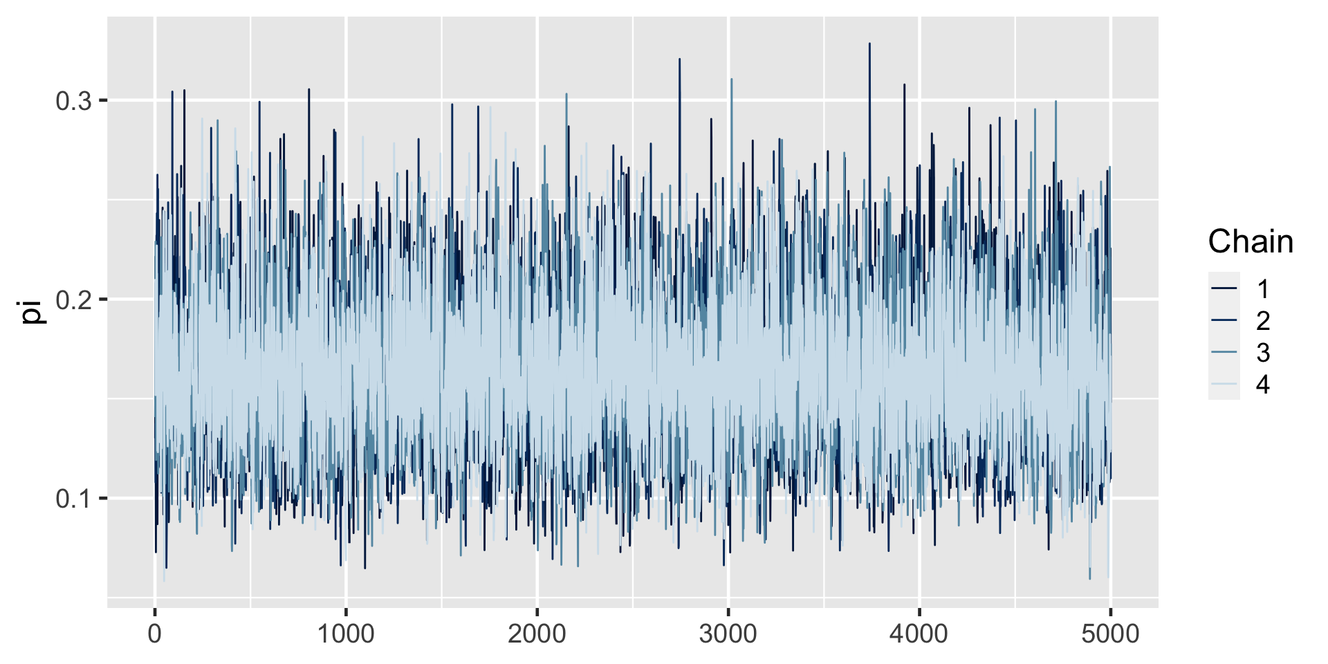

 exceeds     n percent
   FALSE  2987 0.14935
TRUE 17013 0.85065a Bayesian analysis assesses the uncertainty regarding an unknown parameter \(\pi\) in light of observed data \(Y\).
\[P((\pi < 0.20) \; | \; (Y = 14)) = 0.8489856 \;.\]
a frequentist analysis assesses the uncertainty of the observed data \(Y\) in light of assumed values of \(\pi\).
\[P((Y \le 14) | (\pi = 0.20)) = 0.08\]
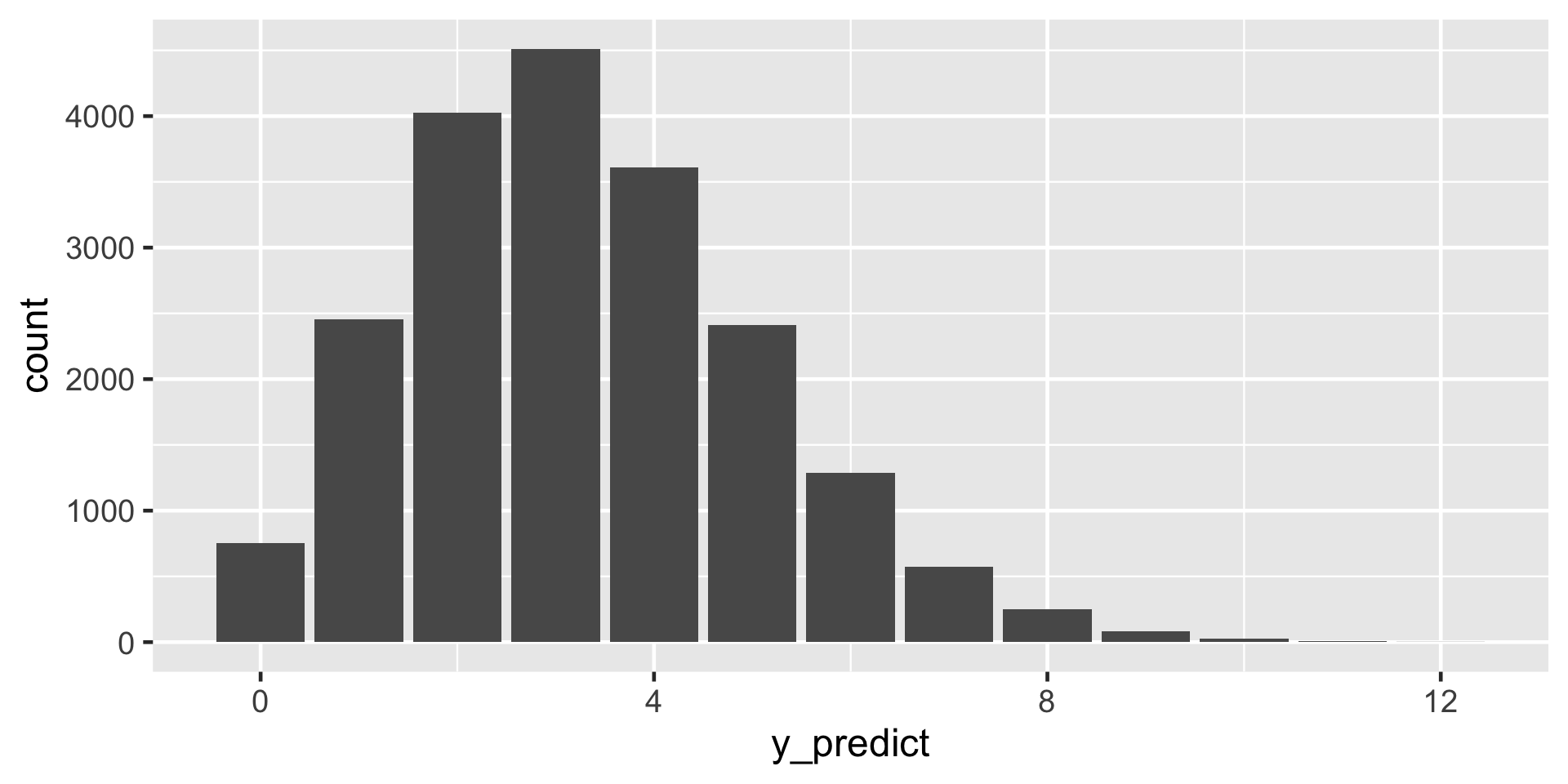
Posterior prediction of new outcomes
Suppose we get our hands on 20 more artworks. What number would you predict are done by artists that are Gen X or younger?
sampling variability
posterior variability in \(\pi\).
First, let \(Y' = y'\) be the (yet unknown) number of the 20 new artworks that are done by Gen X or younger artists. Thus conditioned on \(\pi\), the randomness in \(Y'\) can be modeled by \(Y'|\pi \sim \text{Bin}(20,\pi)\) with pdf
\[f(y'|\pi) = P(Y' = y' | \pi) = \binom{20}{ y'} \pi^{y'}(1-\pi)^{20 - y'}\]
\[f(y'|\pi) f(\pi|(y=14)) \; ,\]
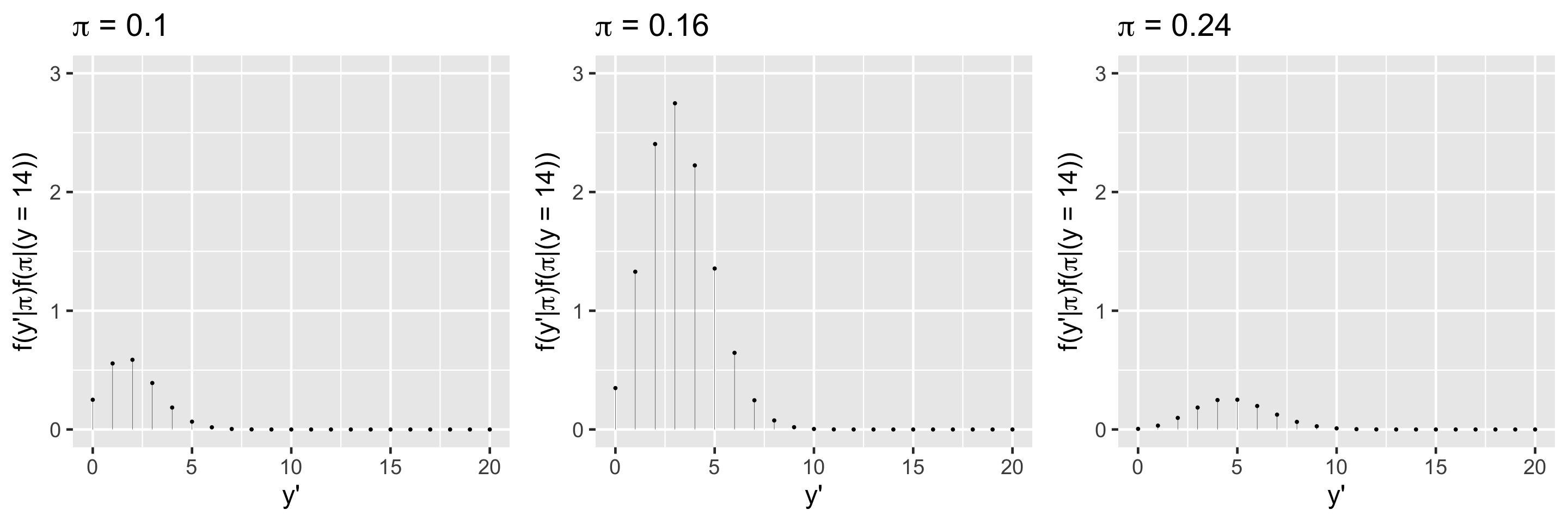
\(f(y'|(y=14)) = \int_0^1 f(y'|\pi) f(\pi|(y=14)) d\pi\)
\(f(y'|(y=14)) = {20 \choose y'} \frac{\Gamma(110)}{\Gamma(18)\Gamma(92)}\frac{\Gamma(18+y')\Gamma(112-y')} {\Gamma(130)} \text{ for } y' \in \{0,1,\ldots,20\}\)
\(f((y'=3)|(y=14)) = {20 \choose 3}\frac{\Gamma(110)}{\Gamma(18)\Gamma(92)}\frac{\Gamma(18+3)\Gamma(112-3)} {\Gamma(130)} = 0.2217\)
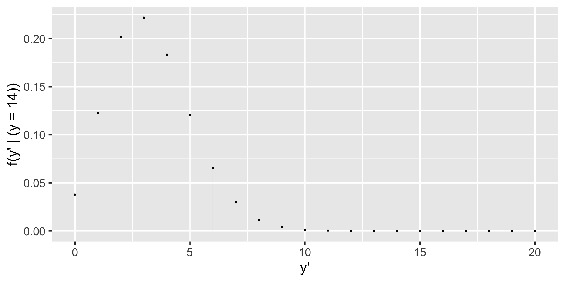
Let \(Y'\) denote a new outcome of variable \(Y\). Further, let pdf \(f(y'|\pi)\) denote the dependence of \(Y'\) on \(\pi\) and posterior pdf \(f(\pi|y)\) denote the posterior plausibility of \(\pi\) given the original data \(Y = y\). Then the posterior predictive model for \(Y'\) has pdf
\[f(y'|y) = \int f(y'|\pi) f(\pi|y) d\pi \; .\]
In words, the overall chance of observing \(Y' = y'\) weights the chance of observing this outcome under any possible \(\pi\) ( \(f(y'|\pi)\) ) by the posterior plausibility of \(\pi\) ( \(f(\pi|y)\) ).
![]()