Summarizing Data

Dr. Mine Dogucu

Summarizing Data with Numbers

We will only summarize a single variable at a time but later we will talk about relationship between two variables.

Summarizing Categorical Data

Categorical data are often summarized with a frequency table. Counts or proportions are used to summarize categorical variables.

	TRUE	FALSE	Total Count
fruity	47	38	85

	TRUE	FALSE	Total Proportion
fruity	0.5529412	0.4470588	1

Summarizing Numerical Data

Consider the following data which represents the number of hours slept for 10 people who were surveyed.

7.5

5.5

7.2

Mean

\[\bar x = \frac{7+7.5+8+5.5+10+7.2+7+8+9+8}{10} = 7.72\]

The mean is calculated by summing the observed values and then dividing by the number of observations.

\[\bar x = \frac{x_1 + x_2+.... x_n}{n}\]

where \(\bar x\) represents the mean of observed values, \(x_1\), \(x_2\), … \(x_n\) represent the n observed values.

Median

If all the observations are listed from smallest to largest (or vice versa), the median is the observation that is in the middle.

5.5

7.2

7.5

In this case, we have two numbers in the middle 7.5 and 8. The average of these numbers would be the median. In this case, the median is 7.75.

\[\frac{7.5 + 8}{2} = 7.75\]

Q1, Q3, and Interquartile Range

You can divide the (ordered) data into four. The median splits the data in half, in other words 50% of the data fall below the median.

First quartile (Q1) is the point at which 25% of the data fall below of. Third quartile (Q3) is the point at which 75% of the data fall below of.

Q1 and Q3 can be considered 25th and 75th percentiles respectively. Interquartile Range (IQR) = Q3 - Q1 which represents the middle 50% of the data.

Quantiles / Percentiles / Quartiles

Quantile	Percentile	Special Name
0.25	25th	First quartile
0.5	50th	Median
0.75	75th	Third quartile

Standard deviation and Variance

Let’s take a detour. Consider Dr. Dogucu teaching three classes. All of these classes have 5 students. Below are midterm results from these classes.

Class 1: 80 80 80 80 80
Class 2: 76 78 80 82 84
Class 3: 60 70 80 90 100

What do you notice about midterm results?

All of these classes have an average of 80 points. But the data differ! In order to explain how these are different we examine how far off each observed value is from the mean on average. In class 1 all students are at the mean value so there is no variance. Class 2 students deviate from the mean slightly on average. Class 3 has the highest deviation from the mean on average.

Standard deviation and Variance

\(x_i\)	\(x_i - \bar{x}\)	\((x_i - \bar{x})^2\)
5.5	5.5-7.72 = -2.22 hr	(-2.2 hr)² = 4.9284 hr ²
7	7-7.72 = -0.72 hr	(-0.72 hr)² = 0.5184 hr ²
7	7-7.72 = -0.72 hr	(-0.72 hr)² = 0.5184 hr ²
7.2	7.2-7.72 = -0.52 hr	(-0.52 hr)² = 0.2704 hr ²
7.5	7.5-7.72 = -0.22 hr	(-0.22 hr)² = 0.0484 hr ²
8	8-7.72 = 0.28 hr	(0.28 hr)² = 0.0784 hr ²
8	8-7.72 = 0.28 hr	(0.28 hr)² = 0.0784 hr ²
8	8-7.72 = 0.28 hr	(0.28 hr)² = 0.0784 hr ²
9	9-7.72 = 1.28 hr	(1.28 hr)² = 1.6384 hr ²
10	10-7.72 = 2.28 hr	(2.28 hr)² = 5.1984 hr ²

Total squared distance from the mean

\(\Sigma_{i = 1}^{n} (x_i - \bar x )^2 =\)

\(4.9284 + 0.5184 + 0.5184 + 0.2704 + 0.0484 +\) \(0.0784 + 0.0784 + 0.0784+ 1.6384 + 5.1984 = 13.356 \text{ hr}^2\)

Note that \(n\) represents the number of observations which means \(n = 10\).

Sample variance

\[s^2 = \frac{\Sigma_{i = 1}^{n} (x_i - \bar x )^2}{n-1}\]

\[s^2= \frac{13.356}{10-1} = 1.484\text{ hr}^2\]

Sample standard deviation

\[s = \sqrt{\frac{\Sigma_{i = 1}^{n} (x_i - \bar x )^2}{n-1}}\]

\[s= \sqrt{1.484} = 1.218195 \text{ hr}\]

Summarizing Data with Numbers in R

Data

glimpse(hotel_bookings)

Rows: 1,000
Columns: 32
$ hotel                          <fct> City Hotel, Resort Hotel, Resort Hotel,…
$ is_canceled                    <fct> 1, 1, 0, 0, 0, 0, 0, 0, 1, 1, 0, 1, 0, …
$ lead_time                      <dbl> 1, 19, 9, 110, 329, 212, 14, 58, 88, 37…
$ arrival_date_year              <dbl> 2015, 2016, 2017, 2016, 2017, 2017, 201…
$ arrival_date_month             <fct> September, March, August, November, Jul…
$ arrival_date_week_number       <dbl> 40, 12, 31, 46, 30, 35, 5, 41, 20, 14, …
$ arrival_date_day_of_month      <dbl> 30, 19, 1, 11, 27, 31, 29, 3, 17, 5, 22…
$ stays_in_weekend_nights        <dbl> 0, 2, 0, 0, 0, 2, 2, 2, 0, 0, 0, 0, 1, …
$ stays_in_week_nights           <dbl> 2, 4, 4, 1, 2, 8, 0, 5, 3, 3, 1, 1, 1, …
$ adults                         <dbl> 1, 2, 2, 2, 2, 2, 1, 2, 2, 2, 1, 2, 1, …
$ children                       <dbl> 0, 0, 0, 0, 0, 1, 0, 0, 0, 0, 0, 0, 0, …
$ babies                         <dbl> 0, 0, 0, 0, 0, 0, 0, 0, 0, 0, 0, 0, 0, …
$ meal                           <fct> BB, BB, HB, BB, SC, BB, BB, BB, SC, BB,…
$ country                        <fct> PRT, PRT, ESP, BRA, GBR, GBR, PRT, DEU,…
$ market_segment                 <fct> Offline TA/TO, Online TA, Online TA, On…
$ distribution_channel           <fct> TA/TO, TA/TO, TA/TO, TA/TO, TA/TO, TA/T…
$ is_repeated_guest              <dbl> 1, 0, 0, 0, 0, 0, 1, 0, 0, 0, 0, 0, 0, …
$ previous_cancellations         <dbl> 1, 0, 0, 0, 0, 0, 0, 0, 0, 0, 0, 0, 0, …
$ previous_bookings_not_canceled <dbl> 0, 0, 0, 0, 0, 0, 1, 0, 0, 0, 0, 0, 0, …
$ reserved_room_type             <fct> A, D, A, A, A, A, A, A, A, A, A, A, A, …
$ assigned_room_type             <fct> A, D, A, A, A, A, D, A, A, A, A, A, A, …
$ booking_changes                <dbl> 0, 0, 0, 2, 0, 1, 0, 0, 0, 0, 0, 0, 1, …
$ deposit_type                   <fct> Non Refund, No Deposit, No Deposit, No …
$ agent                          <fct> 50, 240, 241, 314, 9, 143, 240, 240, 9,…
$ company                        <fct> NULL, NULL, NULL, NULL, NULL, NULL, NUL…
$ days_in_waiting_list           <dbl> 0, 0, 0, 0, 0, 0, 0, 0, 0, 0, 0, 0, 0, …
$ customer_type                  <fct> Transient, Transient, Transient, Transi…
$ average_daily_rate             <dbl> 98.10, 70.17, 193.40, 36.24, 89.10, 89.…
$ required_car_parking_spaces    <dbl> 0, 0, 0, 1, 0, 0, 0, 1, 0, 0, 0, 0, 1, …
$ total_of_special_requests      <dbl> 0, 1, 1, 0, 1, 0, 2, 1, 0, 0, 1, 0, 1, …
$ reservation_status             <fct> Canceled, Canceled, Check-Out, Check-Ou…
$ reservation_status_date        <date> 2015-09-29, 2016-03-02, 2017-08-05, 20…

Data

# A tibble: 1,000 × 2
   is_canceled lead_time
   <fct>           <dbl>
 1 1                   1
 2 1                  19
 3 0                   9
 4 0                 110
 5 0                 329
 6 0                 212
 7 0                  14
 8 0                  58
 9 1                  88
10 1                 373
# ℹ 990 more rows

is_canceled whether the booking was cancelled (0 = FALSE (i.e., not canceled), 1 = TRUE (i.e., canceled))
lead_time number of days between booking and arrival

Summarizing Categorical Data in R

count(hotel_bookings, is_canceled)

# A tibble: 2 × 2
  is_canceled     n
  <fct>       <int>
1 0             634
2 1             366

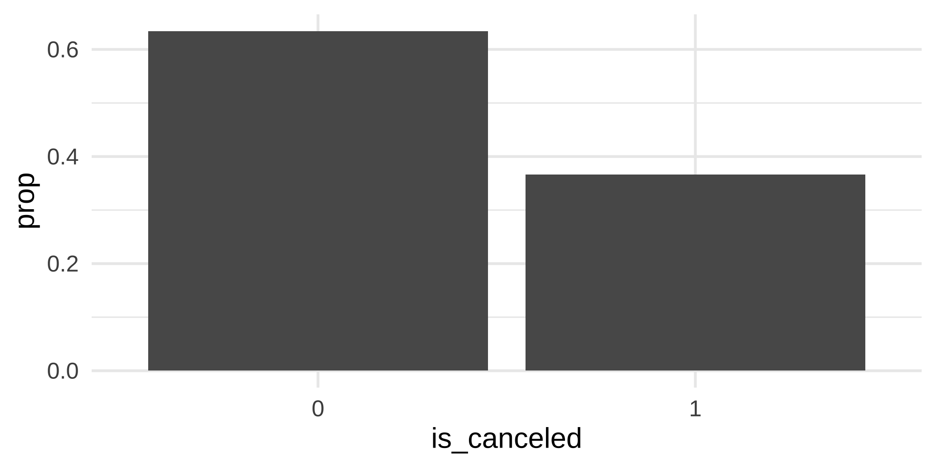
There are 366 people who canceled their booking and 634 who did not.

Summarizing Categorical Data in R

There are total 1000 bookings. We can use this to calculate the proportions

\(\frac{366}{1000}\)

\(\frac{634}{1000}\)

Mean in R

summarize(hotel_bookings, mean(lead_time))

# A tibble: 1 × 1
  `mean(lead_time)`
              <dbl>
1              105.

Median in R

summarize(hotel_bookings, median(lead_time))

# A tibble: 1 × 1
  `median(lead_time)`
                <dbl>
1                69.5

Quartiles

You can specify quartiles (Q3)

summarize(hotel_bookings, quantile(lead_time, 0.75))

# A tibble: 1 × 1
  `quantile(lead_time, 0.75)`
                        <dbl>
1                         157

Standard Deviation and Variance

summarize(hotel_bookings, sd(lead_time))

# A tibble: 1 × 1
  `sd(lead_time)`
            <dbl>
1            106.

summarize(hotel_bookings, var(lead_time))

# A tibble: 1 × 1
  `var(lead_time)`
             <dbl>
1           11331.

Summarizing Data with Visuals

Bar plot with counts

Bar plot with proportions

Histogram

Fun fact

histo comes from the Greek word histos that literally means “anything set up right”.

gram: comes from the Greek word gramma which means “that which is drawn”. ¹

Histogram

Consider the height distribution in our class.

How would the distribution change if Michael Jordan (198.1 cm, 6’ 6’’) were to join our class?
How would the distribution change if Tyrion Lannister (Peter Dinklage) (135 cm, 4’ 5’’) were to join our class?

Note

When data display a skewed distribution we rely on median rather than the mean to understand the center of the distribution.

Exploring Histograms Visually

Boxplot

Median

First and Third Quartiles (Q1 and Q3)

Interquartile Range (IQR)

Whiskers

Whiskers can go as high as Q3 + 1.5 IQR and as low as Q1 - 1.5 IQR. In this instance, we see that whiskers have reached its maximum value, however, since there is no observed data below 0 lead time, the lower whisker is at 0. We can suspect any observed value greater than the maximum reach of whiskers or any observed value less than the minimum reach of whiskers as outliers.

Outliers

Meet Palmer Penguins¹

Data

glimpse(penguins)

Rows: 344
Columns: 8
$ species           <fct> Adelie, Adelie, Adelie, Adelie, Adelie, Adelie, Adel…
$ island            <fct> Torgersen, Torgersen, Torgersen, Torgersen, Torgerse…
$ bill_length_mm    <dbl> 39.1, 39.5, 40.3, NA, 36.7, 39.3, 38.9, 39.2, 34.1, …
$ bill_depth_mm     <dbl> 18.7, 17.4, 18.0, NA, 19.3, 20.6, 17.8, 19.6, 18.1, …
$ flipper_length_mm <int> 181, 186, 195, NA, 193, 190, 181, 195, 193, 190, 186…
$ body_mass_g       <int> 3750, 3800, 3250, NA, 3450, 3650, 3625, 4675, 3475, …
$ sex               <fct> male, female, female, NA, female, male, female, male…
$ year              <int> 2007, 2007, 2007, 2007, 2007, 2007, 2007, 2007, 2007…

What can you conclude from this plot?

Scatterplot

What can you conclude from this plot?

Scatterplot

What can you conclude from this plot?
How many variables are represented in this plot?
Are they numeric or categorical?

Summarizing Data with Visuals in R

Pick your data frame
Pick variables for the axes (or other aesthetics)
Specify the geom (i.e., plot type)

ggplot(hotel_bookings)

ggplot(hotel_bookings, 
       aes(x = lead_time))

ggplot(hotel_bookings, 
       aes(x = lead_time)) +
  geom_histogram()

Box plot

ggplot(penguins, 
       aes(x = species, 
           y = bill_length_mm)) +
  geom_boxplot()

Scatter plot

ggplot(penguins, 
       aes(x = body_mass_g, 
           y = bill_length_mm)) +
  geom_point()

Scatter plot

ggplot(penguins, 
       aes(x = body_mass_g, 
           y = bill_length_mm,
           color = species)) +
  geom_point()

Learning Tip of the Day

Does time management work? A meta-analysis

Summarizing Data

Summarizing Data with Numbers

Summarizing Categorical Data

Summarizing Numerical Data

Mean

Median

Q1, Q3, and Interquartile Range

Quantiles / Percentiles / Quartiles

Standard deviation and Variance

Standard deviation and Variance

Total squared distance from the mean

Sample variance

Sample standard deviation

Summarizing Data with Numbers in R

Data

Data

Summarizing Categorical Data in R

Summarizing Categorical Data in R

Mean in R

Median in R

Quartiles

Standard Deviation and Variance

Summarizing Data with Visuals

Bar plot with counts

Bar plot with proportions

Histogram

Fun fact

Histogram

Note

Boxplot

Median

First and Third Quartiles (Q1 and Q3)

Interquartile Range (IQR)

Whiskers

Outliers

Meet Palmer Penguins1

Data

Scatterplot

Scatterplot

Summarizing Data with Visuals in R

Box plot

Scatter plot

Scatter plot

Learning Tip of the Day

Meet Palmer Penguins¹