Multiple Linear Regression, Transformations, and Model Evaluation

Dr. Mine Dogucu

Data `babies` in `openintro` package

Rows: 1,236
Columns: 8
$ case      <int> 1, 2, 3, 4, 5, 6, 7, 8, 9, 10, 11, 12, 13, 14, 15, 16, 17, 1…
$ bwt       <int> 120, 113, 128, 123, 108, 136, 138, 132, 120, 143, 140, 144, …
$ gestation <int> 284, 282, 279, NA, 282, 286, 244, 245, 289, 299, 351, 282, 2…
$ parity    <int> 0, 0, 0, 0, 0, 0, 0, 0, 0, 0, 0, 0, 0, 0, 0, 0, 0, 0, 0, 0, …
$ age       <int> 27, 33, 28, 36, 23, 25, 33, 23, 25, 30, 27, 32, 23, 36, 30, …
$ height    <int> 62, 64, 64, 69, 67, 62, 62, 65, 62, 66, 68, 64, 63, 61, 63, …
$ weight    <int> 100, 135, 115, 190, 125, 93, 178, 140, 125, 136, 120, 124, 1…
$ smoke     <int> 0, 0, 1, 0, 1, 0, 0, 0, 0, 1, 0, 1, 1, 1, 0, 0, 1, 1, 0, 1, …

y	Response	Birth weight	Numeric
\(x_1\)	Explanatory	Gestation	Numeric
\(x_2\)	Explanatory	Smoke	Categorical

Notation

\(y_i = \beta_0 +\beta_1x_{1i} + \beta_2x_{2i} + \epsilon_i\)

\(\beta_0\) is intercept
\(\beta_1\) is the slope for gestation
\(\beta_2\) is the slope for smoke
\(\epsilon_i\) is error/residual
\(i = 1, 2, ...n\) identifier for each point

model_gs <- lm(bwt ~ gestation + smoke, data = babies)
tidy(model_gs)

# A tibble: 3 × 5
  term        estimate std.error statistic  p.value
  <chr>          <dbl>     <dbl>     <dbl>    <dbl>
1 (Intercept)   -0.932    8.15      -0.114 9.09e- 1
2 gestation      0.443    0.0290    15.3   3.16e-48
3 smoke         -8.09     0.953     -8.49  5.96e-17

Expected birth weight for a baby who had 280 days of gestation with a smoker mother

\(\hat {\text{bwt}_i} = b_0 + b_1 \text{ gestation}_i + b_2 \text{ smoke}_i\)

\(\hat {\text{bwt}_i} = -0.932 + (0.443 \times 280) + (-8.09 \times 1)\)

babies |> 
  modelr::add_predictions(model_gs) |> 
  select(bwt, gestation, smoke, pred)

# A tibble: 1,236 × 4
     bwt gestation smoke  pred
   <int>     <int> <int> <dbl>
 1   120       284     0  125.
 2   113       282     0  124.
 3   128       279     1  115.
 4   123        NA     0   NA 
 5   108       282     1  116.
 6   136       286     0  126.
 7   138       244     0  107.
 8   132       245     0  108.
 9   120       289     0  127.
10   143       299     1  123.
# ℹ 1,226 more rows

babies |> 
  modelr::add_predictions(model_gs) |> 
  modelr::add_residuals(model_gs) |> 
  select(bwt, gestation, smoke, pred, resid)

# A tibble: 1,236 × 5
     bwt gestation smoke  pred  resid
   <int>     <int> <int> <dbl>  <dbl>
 1   120       284     0  125.  -4.84
 2   113       282     0  124. -11.0 
 3   128       279     1  115.  13.5 
 4   123        NA     0   NA   NA   
 5   108       282     1  116.  -7.87
 6   136       286     0  126.  10.3 
 7   138       244     0  107.  30.9 
 8   132       245     0  108.  24.4 
 9   120       289     0  127.  -7.05
10   143       299     1  123.  19.6 
# ℹ 1,226 more rows

Transformations

Data

library(AmesHousing)
ames_raw <- janitor::clean_names(ames_raw)
glimpse(ames_raw)

Rows: 2,930
Columns: 82
$ order           <int> 1, 2, 3, 4, 5, 6, 7, 8, 9, 10, 11, 12, 13, 14, 15, 16,…
$ pid             <chr> "0526301100", "0526350040", "0526351010", "0526353030"…
$ ms_sub_class    <chr> "020", "020", "020", "020", "060", "060", "120", "120"…
$ ms_zoning       <chr> "RL", "RH", "RL", "RL", "RL", "RL", "RL", "RL", "RL", …
$ lot_frontage    <int> 141, 80, 81, 93, 74, 78, 41, 43, 39, 60, 75, NA, 63, 8…
$ lot_area        <int> 31770, 11622, 14267, 11160, 13830, 9978, 4920, 5005, 5…
$ street          <chr> "Pave", "Pave", "Pave", "Pave", "Pave", "Pave", "Pave"…
$ alley           <chr> NA, NA, NA, NA, NA, NA, NA, NA, NA, NA, NA, NA, NA, NA…
$ lot_shape       <chr> "IR1", "Reg", "IR1", "Reg", "IR1", "IR1", "Reg", "IR1"…
$ land_contour    <chr> "Lvl", "Lvl", "Lvl", "Lvl", "Lvl", "Lvl", "Lvl", "HLS"…
$ utilities       <chr> "AllPub", "AllPub", "AllPub", "AllPub", "AllPub", "All…
$ lot_config      <chr> "Corner", "Inside", "Corner", "Corner", "Inside", "Ins…
$ land_slope      <chr> "Gtl", "Gtl", "Gtl", "Gtl", "Gtl", "Gtl", "Gtl", "Gtl"…
$ neighborhood    <chr> "NAmes", "NAmes", "NAmes", "NAmes", "Gilbert", "Gilber…
$ condition_1     <chr> "Norm", "Feedr", "Norm", "Norm", "Norm", "Norm", "Norm…
$ condition_2     <chr> "Norm", "Norm", "Norm", "Norm", "Norm", "Norm", "Norm"…
$ bldg_type       <chr> "1Fam", "1Fam", "1Fam", "1Fam", "1Fam", "1Fam", "Twnhs…
$ house_style     <chr> "1Story", "1Story", "1Story", "1Story", "2Story", "2St…
$ overall_qual    <int> 6, 5, 6, 7, 5, 6, 8, 8, 8, 7, 6, 6, 6, 7, 8, 8, 8, 9, …
$ overall_cond    <int> 5, 6, 6, 5, 5, 6, 5, 5, 5, 5, 5, 7, 5, 5, 5, 5, 7, 2, …
$ year_built      <int> 1960, 1961, 1958, 1968, 1997, 1998, 2001, 1992, 1995, …
$ year_remod_add  <int> 1960, 1961, 1958, 1968, 1998, 1998, 2001, 1992, 1996, …
$ roof_style      <chr> "Hip", "Gable", "Hip", "Hip", "Gable", "Gable", "Gable…
$ roof_matl       <chr> "CompShg", "CompShg", "CompShg", "CompShg", "CompShg",…
$ exterior_1st    <chr> "BrkFace", "VinylSd", "Wd Sdng", "BrkFace", "VinylSd",…
$ exterior_2nd    <chr> "Plywood", "VinylSd", "Wd Sdng", "BrkFace", "VinylSd",…
$ mas_vnr_type    <chr> "Stone", "None", "BrkFace", "None", "None", "BrkFace",…
$ mas_vnr_area    <int> 112, 0, 108, 0, 0, 20, 0, 0, 0, 0, 0, 0, 0, 0, 0, 603,…
$ exter_qual      <chr> "TA", "TA", "TA", "Gd", "TA", "TA", "Gd", "Gd", "Gd", …
$ exter_cond      <chr> "TA", "TA", "TA", "TA", "TA", "TA", "TA", "TA", "TA", …
$ foundation      <chr> "CBlock", "CBlock", "CBlock", "CBlock", "PConc", "PCon…
$ bsmt_qual       <chr> "TA", "TA", "TA", "TA", "Gd", "TA", "Gd", "Gd", "Gd", …
$ bsmt_cond       <chr> "Gd", "TA", "TA", "TA", "TA", "TA", "TA", "TA", "TA", …
$ bsmt_exposure   <chr> "Gd", "No", "No", "No", "No", "No", "Mn", "No", "No", …
$ bsmt_fin_type_1 <chr> "BLQ", "Rec", "ALQ", "ALQ", "GLQ", "GLQ", "GLQ", "ALQ"…
$ bsmt_fin_sf_1   <int> 639, 468, 923, 1065, 791, 602, 616, 263, 1180, 0, 0, 9…
$ bsmt_fin_type_2 <chr> "Unf", "LwQ", "Unf", "Unf", "Unf", "Unf", "Unf", "Unf"…
$ bsmt_fin_sf_2   <int> 0, 144, 0, 0, 0, 0, 0, 0, 0, 0, 0, 0, 0, 0, 1120, 0, 0…
$ bsmt_unf_sf     <int> 441, 270, 406, 1045, 137, 324, 722, 1017, 415, 994, 76…
$ total_bsmt_sf   <int> 1080, 882, 1329, 2110, 928, 926, 1338, 1280, 1595, 994…
$ heating         <chr> "GasA", "GasA", "GasA", "GasA", "GasA", "GasA", "GasA"…
$ heating_qc      <chr> "Fa", "TA", "TA", "Ex", "Gd", "Ex", "Ex", "Ex", "Ex", …
$ central_air     <chr> "Y", "Y", "Y", "Y", "Y", "Y", "Y", "Y", "Y", "Y", "Y",…
$ electrical      <chr> "SBrkr", "SBrkr", "SBrkr", "SBrkr", "SBrkr", "SBrkr", …
$ x1st_flr_sf     <int> 1656, 896, 1329, 2110, 928, 926, 1338, 1280, 1616, 102…
$ x2nd_flr_sf     <int> 0, 0, 0, 0, 701, 678, 0, 0, 0, 776, 892, 0, 676, 0, 0,…
$ low_qual_fin_sf <int> 0, 0, 0, 0, 0, 0, 0, 0, 0, 0, 0, 0, 0, 0, 0, 0, 0, 0, …
$ gr_liv_area     <int> 1656, 896, 1329, 2110, 1629, 1604, 1338, 1280, 1616, 1…
$ bsmt_full_bath  <int> 1, 0, 0, 1, 0, 0, 1, 0, 1, 0, 0, 1, 0, 1, 1, 1, 0, 1, …
$ bsmt_half_bath  <int> 0, 0, 0, 0, 0, 0, 0, 0, 0, 0, 0, 0, 0, 0, 0, 0, 0, 0, …
$ full_bath       <int> 1, 1, 1, 2, 2, 2, 2, 2, 2, 2, 2, 2, 2, 1, 1, 3, 2, 1, …
$ half_bath       <int> 0, 0, 1, 1, 1, 1, 0, 0, 0, 1, 1, 0, 1, 1, 1, 1, 0, 1, …
$ bedroom_abv_gr  <int> 3, 2, 3, 3, 3, 3, 2, 2, 2, 3, 3, 3, 3, 2, 1, 4, 4, 1, …
$ kitchen_abv_gr  <int> 1, 1, 1, 1, 1, 1, 1, 1, 1, 1, 1, 1, 1, 1, 1, 1, 1, 1, …
$ kitchen_qual    <chr> "TA", "TA", "Gd", "Ex", "TA", "Gd", "Gd", "Gd", "Gd", …
$ tot_rms_abv_grd <int> 7, 5, 6, 8, 6, 7, 6, 5, 5, 7, 7, 6, 7, 5, 4, 12, 8, 8,…
$ functional      <chr> "Typ", "Typ", "Typ", "Typ", "Typ", "Typ", "Typ", "Typ"…
$ fireplaces      <int> 2, 0, 0, 2, 1, 1, 0, 0, 1, 1, 1, 0, 1, 1, 0, 1, 0, 1, …
$ fireplace_qu    <chr> "Gd", NA, NA, "TA", "TA", "Gd", NA, NA, "TA", "TA", "T…
$ garage_type     <chr> "Attchd", "Attchd", "Attchd", "Attchd", "Attchd", "Att…
$ garage_yr_blt   <int> 1960, 1961, 1958, 1968, 1997, 1998, 2001, 1992, 1995, …
$ garage_finish   <chr> "Fin", "Unf", "Unf", "Fin", "Fin", "Fin", "Fin", "RFn"…
$ garage_cars     <int> 2, 1, 1, 2, 2, 2, 2, 2, 2, 2, 2, 2, 2, 2, 2, 3, 2, 3, …
$ garage_area     <int> 528, 730, 312, 522, 482, 470, 582, 506, 608, 442, 440,…
$ garage_qual     <chr> "TA", "TA", "TA", "TA", "TA", "TA", "TA", "TA", "TA", …
$ garage_cond     <chr> "TA", "TA", "TA", "TA", "TA", "TA", "TA", "TA", "TA", …
$ paved_drive     <chr> "P", "Y", "Y", "Y", "Y", "Y", "Y", "Y", "Y", "Y", "Y",…
$ wood_deck_sf    <int> 210, 140, 393, 0, 212, 360, 0, 0, 237, 140, 157, 483, …
$ open_porch_sf   <int> 62, 0, 36, 0, 34, 36, 0, 82, 152, 60, 84, 21, 75, 0, 5…
$ enclosed_porch  <int> 0, 0, 0, 0, 0, 0, 170, 0, 0, 0, 0, 0, 0, 0, 0, 0, 0, 0…
$ x3ssn_porch     <int> 0, 0, 0, 0, 0, 0, 0, 0, 0, 0, 0, 0, 0, 0, 0, 0, 0, 0, …
$ screen_porch    <int> 0, 120, 0, 0, 0, 0, 0, 144, 0, 0, 0, 0, 0, 0, 140, 210…
$ pool_area       <int> 0, 0, 0, 0, 0, 0, 0, 0, 0, 0, 0, 0, 0, 0, 0, 0, 0, 0, …
$ pool_qc         <chr> NA, NA, NA, NA, NA, NA, NA, NA, NA, NA, NA, NA, NA, NA…
$ fence           <chr> NA, "MnPrv", NA, NA, "MnPrv", NA, NA, NA, NA, NA, NA, …
$ misc_feature    <chr> NA, NA, "Gar2", NA, NA, NA, NA, NA, NA, NA, NA, "Shed"…
$ misc_val        <int> 0, 0, 12500, 0, 0, 0, 0, 0, 0, 0, 0, 500, 0, 0, 0, 0, …
$ mo_sold         <int> 5, 6, 6, 4, 3, 6, 4, 1, 3, 6, 4, 3, 5, 2, 6, 6, 6, 6, …
$ yr_sold         <int> 2010, 2010, 2010, 2010, 2010, 2010, 2010, 2010, 2010, …
$ sale_type       <chr> "WD ", "WD ", "WD ", "WD ", "WD ", "WD ", "WD ", "WD "…
$ sale_condition  <chr> "Normal", "Normal", "Normal", "Normal", "Normal", "Nor…
$ sale_price      <int> 215000, 105000, 172000, 244000, 189900, 195500, 213500…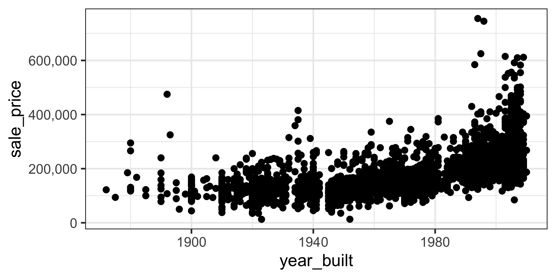

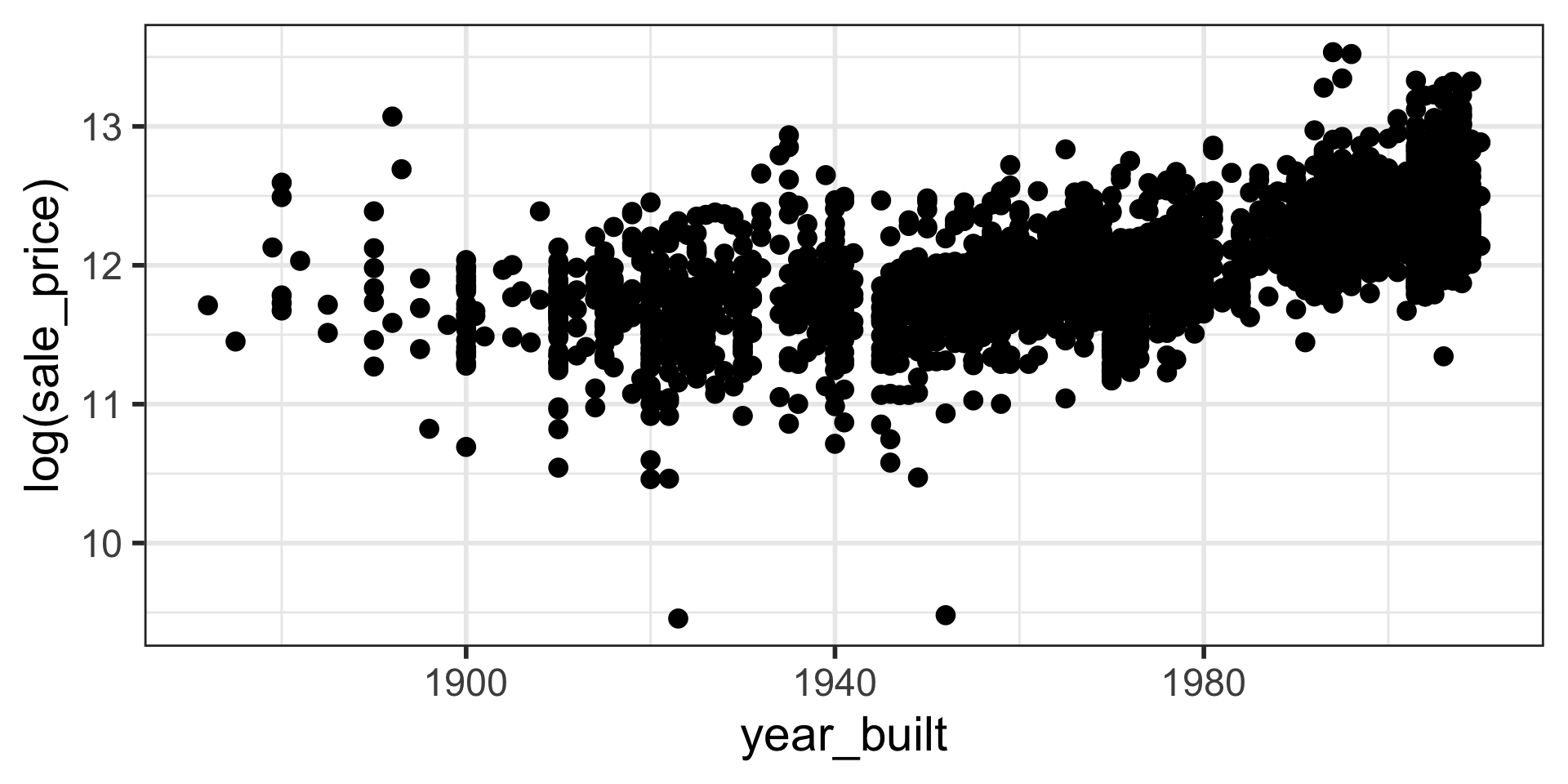
Note that log is natural log in R.

model_y <- lm(log(sale_price) ~ year_built, 
              data = ames_raw)
tidy(model_y)

# A tibble: 2 × 5
  term        estimate std.error statistic   p.value
  <chr>          <dbl>     <dbl>     <dbl>     <dbl>
1 (Intercept) -4.33     0.387        -11.2 1.73e- 28
2 year_built   0.00829  0.000196      42.3 4.45e-305

\({log(\hat y_i)} = b_0 + b_1x_{1i}\)

\({log(\hat y_i)} = -4.33 + 0.00829x_{1i}\)

Estimated sale price of a house built in 1980

\({log(\hat y_i)} = -4.33 + 0.00829 \times 1980\)

\(e^{log(\hat y_i)} = e^{-4.33 + 0.00829 \times 1980}\)

\(\hat y_i = e^{-4.33} \times e^ {0.00829 \times 1980} = 177052.2\)

For one-unit (year) increase in x, the y is multiplied by \(e^{b_1}\).

Note that \(e^x\) can be achieved by exp(x) in R.

When Relationships Aren’t Linear: Transformations

Linear regression models assume a linear relationship between the explanatory (X) and response (Y) variables.
What if the real relationship is curved (non-linear)?
We can transform our variables to make the relationship linear, allowing us to still use linear regression.

Common Transformations

Logarithmic: log(Y) or log(X). Useful when a variable has a wide range of values or a skewed distribution (like housing prices).
Reciprocal: 1/Y or 1/X
Square Root: sqrt(Y) or sqrt(X)

Model Evaluation

glimpse(babies)

Rows: 1,236
Columns: 8
$ case      <int> 1, 2, 3, 4, 5, 6, 7, 8, 9, 10, 11, 12, 13, 14, 15, 16, 17, 1…
$ bwt       <int> 120, 113, 128, 123, 108, 136, 138, 132, 120, 143, 140, 144, …
$ gestation <int> 284, 282, 279, NA, 282, 286, 244, 245, 289, 299, 351, 282, 2…
$ parity    <int> 0, 0, 0, 0, 0, 0, 0, 0, 0, 0, 0, 0, 0, 0, 0, 0, 0, 0, 0, 0, …
$ age       <int> 27, 33, 28, 36, 23, 25, 33, 23, 25, 30, 27, 32, 23, 36, 30, …
$ height    <int> 62, 64, 64, 69, 67, 62, 62, 65, 62, 66, 68, 64, 63, 61, 63, …
$ weight    <int> 100, 135, 115, 190, 125, 93, 178, 140, 125, 136, 120, 124, 1…
$ smoke     <int> 0, 0, 1, 0, 1, 0, 0, 0, 0, 1, 0, 1, 1, 1, 0, 0, 1, 1, 0, 1, …

model_g <- lm(bwt ~ gestation, data = babies)
tidy(model_g)

# A tibble: 2 × 5
  term        estimate std.error statistic  p.value
  <chr>          <dbl>     <dbl>     <dbl>    <dbl>
1 (Intercept)  -10.1      8.32       -1.21 2.27e- 1
2 gestation      0.464    0.0297     15.6  3.22e-50

glance(model_g)

# A tibble: 1 × 12
  r.squared adj.r.squared sigma statistic  p.value    df logLik    AIC    BIC
      <dbl>         <dbl> <dbl>     <dbl>    <dbl> <dbl>  <dbl>  <dbl>  <dbl>
1     0.166         0.166  16.7      244. 3.22e-50     1 -5175. 10356. 10371.
# ℹ 3 more variables: deviance <dbl>, df.residual <int>, nobs <int>

glance(model_g)$r.squared

[1] 0.1663449

16% of the variation in birth weight is explained by gestation. Higher values of R squared is preferred.

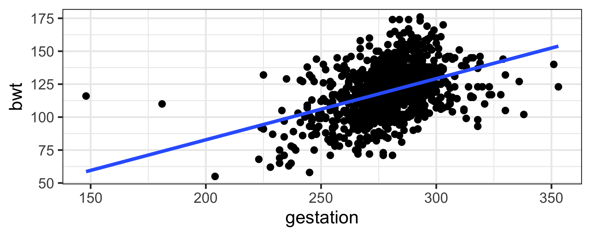
\(R\) and \(R^2\)

\(R^2\) = 0.1663449

\(b_1 = \frac{s_y}{s_x}R\)

\(R\) is the correlation coefficient

model_gsa <- lm(bwt ~ gestation + smoke + age, data = babies)

The Problem with Adding More Variables

Every time you add a variable to a model, the regular R-squared will always increase (or stay the same), even if the variable is useless.
This can trick us into building an overly complex model that is “memorizing” our sample data instead of learning the true underlying patterns. This is called overfitting (more on this later).
An overfit model performs well on the data it was trained on, but fails when it sees new, unseen data.

A Better Metric: Adjusted R-Squared

Adjusted R-squared penalizes the model for having extra variables that don’t contribute meaningfully.
It only increases if the new variable improves the model more than would be expected by chance.
Rule of Thumb: When comparing models with different numbers of variables, always prefer the one with the higher Adjusted R-squared.

Adjusted R-Squared

glance(model_g)

# A tibble: 1 × 12
  r.squared adj.r.squared sigma statistic  p.value    df logLik    AIC    BIC
      <dbl>         <dbl> <dbl>     <dbl>    <dbl> <dbl>  <dbl>  <dbl>  <dbl>
1     0.166         0.166  16.7      244. 3.22e-50     1 -5175. 10356. 10371.
# ℹ 3 more variables: deviance <dbl>, df.residual <int>, nobs <int>

glance(model_gsa)

# A tibble: 1 × 12
  r.squared adj.r.squared sigma statistic  p.value    df logLik    AIC    BIC
      <dbl>         <dbl> <dbl>     <dbl>    <dbl> <dbl>  <dbl>  <dbl>  <dbl>
1     0.212         0.210  16.2      108. 3.45e-62     3 -5089. 10187. 10213.
# ℹ 3 more variables: deviance <dbl>, df.residual <int>, nobs <int>

When comparing models with multiple predictors we rely on Adjusted R-squared.

Model Selection and Occam’s Razor

“Among competing hypotheses, the one with the fewest assumptions should be selected.”

How does this apply to our models?

Simpler is Better: A model with fewer variables (a simpler model) is preferable to a complex model if they both have similar predictive power (similar Adjusted R-squared).
Why?
1. Avoids Overfitting: Simpler models are less likely to be overfit to the sample data and will generalize better to new data.
2. Easier to Interpret: It’s much easier to understand the relationship between 3 variables and birth weight than between 10 variables and birth weight.

Occam’s Razor provides the philosophical foundation for why we use techniques like Adjusted R-squared and Train/Test splitting: to find the simplest model that does the best job.

babies |> 
  add_predictions(model_g) |> 
  add_residuals(model_g) |> 
  select(bwt, pred, resid)

# A tibble: 1,236 × 3
     bwt  pred  resid
   <int> <dbl>  <dbl>
 1   120  122.  -1.79
 2   113  121.  -7.86
 3   128  119.   8.53
 4   123   NA   NA   
 5   108  121. -12.9 
 6   136  123.  13.3 
 7   138  103.  34.8 
 8   132  104.  28.3 
 9   120  124.  -4.11
10   143  129.  14.2 
# ℹ 1,226 more rows

babies |> 
  add_predictions(model_gsa) |> 
  add_residuals(model_gsa) |> 
  select(bwt, pred, resid)

# A tibble: 1,236 × 3
     bwt  pred  resid
   <int> <dbl>  <dbl>
 1   120  125.  -4.80
 2   113  125. -11.5 
 3   128  115.  13.3 
 4   123   NA   NA   
 5   108  115.  -7.47
 6   136  125.  10.5 
 7   138  108.  30.4 
 8   132  107.  25.0 
 9   120  127.  -6.81
10   143  124.  19.2 
# ℹ 1,226 more rows

Root Mean Square Error

\(RMSE = \sqrt{\frac{\Sigma_{i=1}^n(y_i-\hat y_i)^2}{n}}\)

modelr::rmse(model_gsa, babies)

[1] 16.1687

modelr::rmse(model_g, babies)

[1] 16.6512

model_full <- lm(bwt ~ gestation + parity + age +
                   height + weight + smoke, 
                 data = babies)

modelr::rmse(model_full, babies)

[1] 15.78198

glance(model_full)$adj.r.squared

[1] 0.2541383

Can we keep adding all the variables and try to get an EXCELLENT model fit?

Overfitting

We are fitting the model to sample data.
Our goal is to understand the population data.
If we make our model too perfect for our sample data, the model may not perform as well with other sample data from the population.
In this case we would be overfitting the data.
We can use model validation techniques.

Splitting the Data (Train vs. Test)

set.seed(12345)
babies_split <- rsample::initial_split(babies) ## 75% to 25% split

babies_train <- rsample::training(babies_split)
dim(babies_train)

[1] 927   8

babies_test <- rsample::testing(babies_split)
dim(babies_test)

[1] 309   8

model_gsa_train <- lm(bwt ~ gestation + smoke + age, data = babies_train)
model_gsa_test <- lm(bwt ~ gestation + smoke + age, data = babies_test)

glance(model_gsa_train)

# A tibble: 1 × 12
  r.squared adj.r.squared sigma statistic  p.value    df logLik   AIC   BIC
      <dbl>         <dbl> <dbl>     <dbl>    <dbl> <dbl>  <dbl> <dbl> <dbl>
1     0.204         0.201  16.4      76.8 2.87e-44     3 -3815. 7641. 7665.
# ℹ 3 more variables: deviance <dbl>, df.residual <int>, nobs <int>

glance(model_gsa_test)

# A tibble: 1 × 12
  r.squared adj.r.squared sigma statistic  p.value    df logLik   AIC   BIC
      <dbl>         <dbl> <dbl>     <dbl>    <dbl> <dbl>  <dbl> <dbl> <dbl>
1     0.243         0.236  15.8      32.2 4.21e-18     3 -1272. 2553. 2572.
# ℹ 3 more variables: deviance <dbl>, df.residual <int>, nobs <int>

modelr::rmse(model_gsa_train, babies_train)

[1] 16.31741

modelr::rmse(model_gsa_test, babies_test)

[1] 15.64897

Exercises

8.12
9.4
9.10